Dimensionality Reduction using Auto-Encoders

Imagine having over thousands of input features in your dataset and you've to train them all..well, sometimes we wish we could compress the dataset to less number of features. Right? well, we can do that using a special type of Neural Network called Auto-encoders. So, let's have a brief introduction to Auto-encoders.

What in the world are Auto-encoders

Auto-encoders are a branch of neural networks which basically compresses the information of the input variables into a reduced dimensional space and then it recreate the input data set to train it all over again.

Auto-encoder consists of 3 main components

• Encoder
• Code
• Decoder

Encoder: An encoder is a feed-forward, fully connected neural network that compresses the input into a latent space representation and encodes the input image as a compressed representation in a reduced dimension, and produces code. The lower the size of the code, the higher the compression.

Code: This part of the network contains the reduced representation of the input that is fed into the decoder.

Decoder: A decoder is also a feed-forward neural network that is similar to an encoder but the representation is the exact mirror image of the encoder. The decoder reconstructs the input back to the original dimensions from the code.

Note: The dimensions of both input and output must be the same.

first, the input passes through the encoder, which is a fully-connected ANN, to produce the code. The decoder, which has the similar ANN structure, then produces the output only using the code. The goal is to get an output identical with the input. Note that the decoder architecture is the mirror image of the encoder. This is not a requirement but it's typically the case. The only requirement is the dimensionality of the input and output needs to be the same. Anything in the middle can be played with.

Hyperparameters

Auto Encoders can have many different hyperparameters but the very important ones are:

• Code size: number of nodes in the middle layer. Smaller size results in more compression.
• Number of layers: the auto-encoder can be as deep as we like. In the figure above we have 2 layers in both the encoder and decoder, without considering the input and output.
• Number of nodes per layer: the auto-encoder architecture we're working on is called a stacked auto-encoder since the layers are stacked one after another. Usually stacked autoencoders look like a "sandwich". The number of nodes per layer decreases with each subsequent layer of the encoder and increases back in the decoder. Also, the decoder is symmetric to the encoder in terms of the layer structure. As noted above this is not necessary and we have total control over these parameters.
• Loss function: we either use mean squared error (mse) or binary cross-entropy. If the input values are in the range [0, 1] then we typically use cross-entropy, otherwise, we use the mean squared error.

Code Implementation

Let's look at how we can do dimensionality reduction using auto-encoders. Let's take a dataset that has 12 features and 8664 columns. Now our goal is to compress the dataset into 6 features.

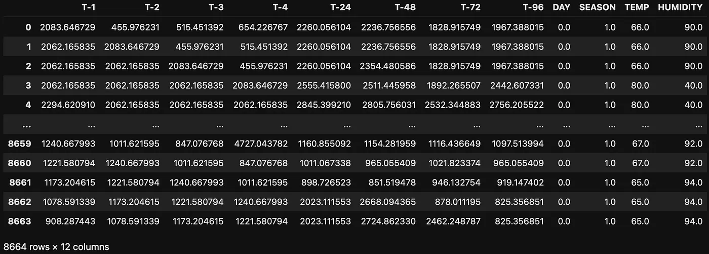
Original dataset with 12 features

Let us scale the data so that all our data points lie in the same range

        from sklearn.preprocessing import MinMaxScaler
scaler = MinMaxScaler()
df_scaled = scaler.fit_transform(df)
X_train_df = pd.DataFrame(df_scaled, columns=df.columns)
X_train_df
    

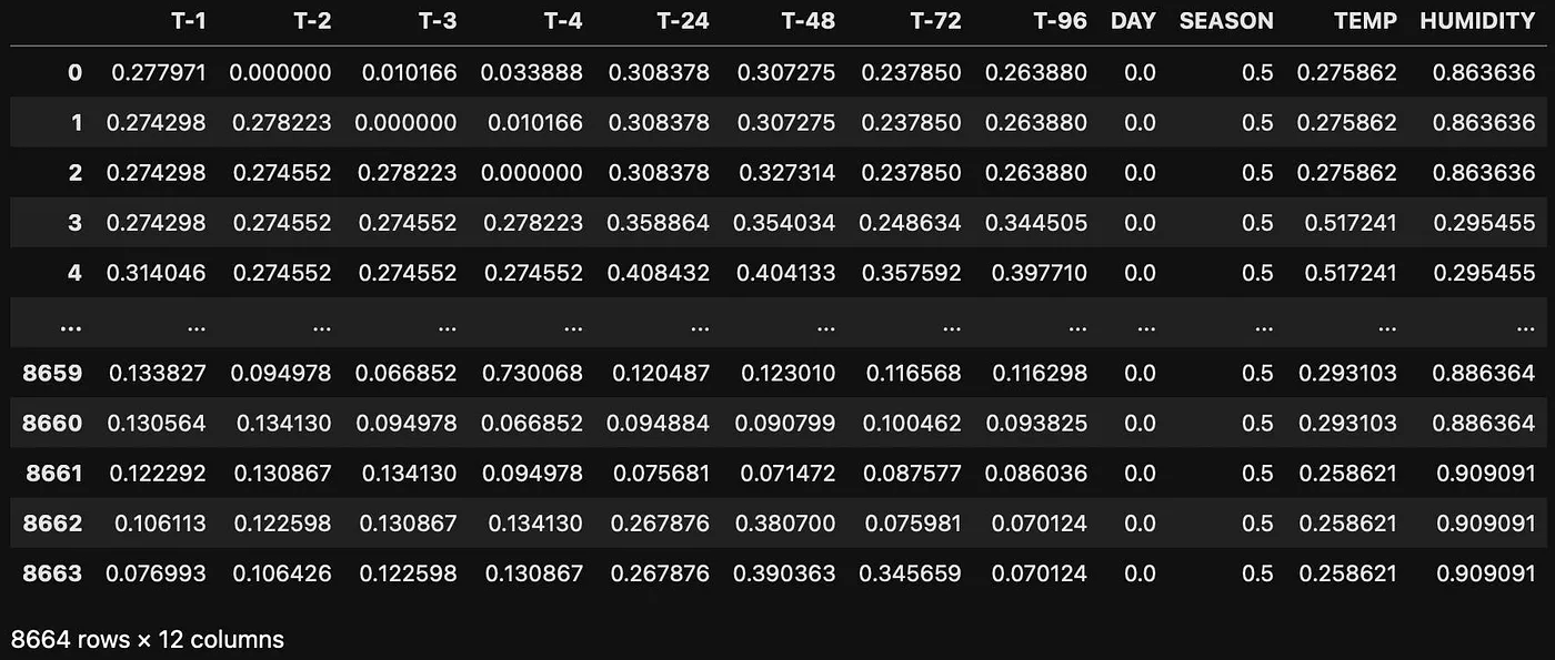
dataset after scaling

Let's build an auto-encoder with a code size of 6.

        import tensorflow as tf 
from tensorflow.keras.layers import Input, Dense
from tensorflow.keras.models import Model
# 12, 11, 10, 9, 8, 7, 6, 7, 8, 9, 10, 11, 12
 
# encoder
encoder_input = Input(shape=(n_features), name='encoder_input')
encoder_layer1 = Dense(11, activation='relu', name='encoder_layer1')(encoder_input)
encoder_layer2 = Dense(10, activation='relu', name='encoder_layer2')(encoder_layer1)
encoder_layer3 = Dense(9, activation='relu', name='encoder_layer3')(encoder_layer2)
encoder_layer4 = Dense(8, activation='relu', name='encoder_layer4')(encoder_layer3)
encoder_layer5 = Dense(7, activation='relu', name='encoder_layer5')(encoder_layer4)
latent_space = Dense(6, activation='relu', name='latent_space')(encoder_layer5)
 
#decoder
decoder_layer1 = Dense(7, activation='relu', name='decoder_layer1')(latent_space)
decoder_layer2 = Dense(8, activation='relu', name='decoder_layer2')(decoder_layer1)
decoder_layer3 = Dense(9, activation='relu', name='decoder_layer3')(decoder_layer2)
decoder_layer4 = Dense(10, activation='relu', name='decoder_layer4')(decoder_layer3)
decoder_layer5 = Dense(11, activation='relu', name='decoder_layer5')(decoder_layer4)
output = Dense(n_features, activation='sigmoid', name='Output')(decoder_layer5)
autoencoder = Model(encoder_input, output, name='Autoencoder')
 
autoencoder.compile(optimizer='adam',
                    loss=tf.keras.losses.mean_squared_error)
autoencoder.summary()
    

let's train the model

        history = autoencoder.fit(X_train_df,
                          X_train_df,
                          epochs=100,
                          steps_per_epoch=10,
                          verbose=0)
# only the encoder part
encoder = Model(inputs=encoder_input, outputs=latent_space)
encoder.compile(optimizer='adam',
                        loss=tf.keras.losses.mean_squared_error)
X_train_encode = encoder.predict(X_train_df)
encoded_train = pd.DataFrame(X_train_encode,
                             columns=[f"X{x}" for x in range(1, X_train_encode.shape[1]+1)])
    

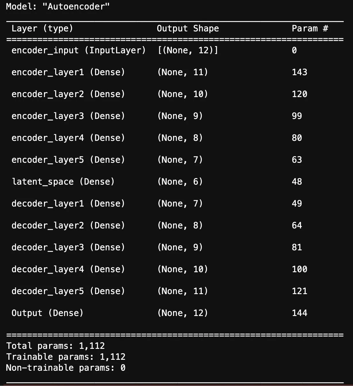
autoencoder model summary

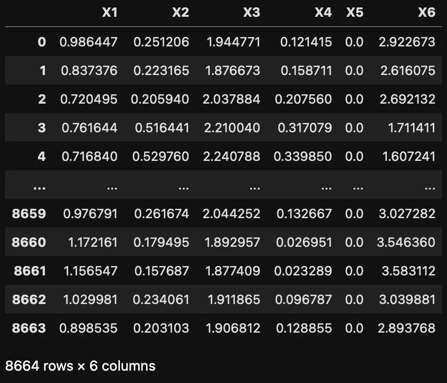
Compressed version of the original (12 features) dataset with 6 features

We can see that output from the encoder which compressed our dataset into 6 features.

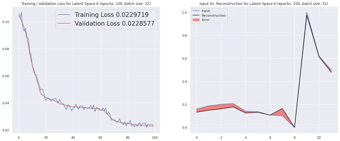
Input Vs. Reconstruction plot. The red shaded portion shows the error between Original vs Reconstructed data.